Generated using Microsoft Bing Image Generator
Overview of Generative Models
In simple terms, generative models are machine learning models that model the training data distribution and generate new samples. Mathematically, a generative model can learn the distribution p(x) which closely approximates the true data distribution q(x) based on the evidence or data X. When using a parametric model to learn p(x), this problem transforms to maximizing the average log-likelihood of the samples x with respect to the parameters.

Equation 1
In this series of articles, we will learn about the Diffusion-based Generative models which draw their inspiration from non-equilibrium thermodynamics.
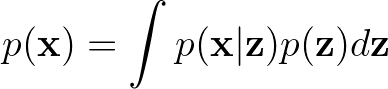
Generative models like GAN, and VAE models only approximate the data distribution as calculating the data distribution p(x) from the latent vectors is often intractable.
Equation 2
In Normalizing Flow-based models, crafting specialized architectures for invertible transforms often poses problems for easy applicability.
Generative Model Paradigms (GAN, VAE, Normalizing Flows)
At the end of the day, generative models are judged based on the ease of training them to generate good samples. All generative models, be it GANs, VAE or Diffusion Models, can map a random sample drawn from a noise distribution to a sample from the data distribution q(x).
- GAN draws a random sample from a noise distribution N(0, I) and generates an image or sample using the Generator G(x|z), which is discriminated by the Discriminator D(x) as real or fake. Thus, the job of the Generator is to map samples from N(0, I) to p(x) which approximates q(x).
- VAE learns the mapping from a prior distribution N(0, I) to the true input distribution q(x). However, as in Eqn. 2 above, approximating q(x) using p(x) becomes intractable due to the presence of p(z). Trying to sample p(z|x) is also intractable. Due to the intractability of the posterior distribution p(z|x) in deep latent variable models, a parametrized conditional distribution q(z|x) is used.
- Normalizing Flow models a sequence of transformations to learn the mapping from a prior distribution N(0, I) to the data distribution p(x).
What is common in all the above models is that those models map a prior distribution N(0, I) to the data distribution q(x) by maximizing the log-likelihood of the parametric approximation of the data distribution, i.e., p(x).
Likelihood and Why We Maximize It
A likelihood function measures how well a statistical model explains the observed data. It measures how “likely” any particular value of a parameter is for any particular value of the observation X = x.

Equation 3: Likelihood Function
where p(x|theta) denotes the joint probability distribution function of the sample X. The function L(theta|x) is called the likelihood function.
If we compare the likelihood function at two points in the parameter space, then find that,

Equation 4
Then, we can say that the observation X = x is more likely to be observed for \theta_1 than \theta_2. In other words, \theta_1 is more plausible than \theta_2. The likelihood function actually considers x to be a observed value, whereas \theta is varied over the whole of the parameter space.
Thus, to learn the true distribution of the data q(x) it is necessary to maximize this likelihood of the data given by Eqn. (3).
This aspect of the likelihood function is utilized in Diffusion models by maximizing the likelihood through estimatation of the score.
However, even though p(x|\theta) is a pdf gives us a probability of the the observed value x given the parameter values \theta, there is no guarantee that L(\theta|x) is a pdf.
What is Score?
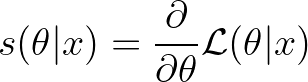
The score (or Informant) in statistics is the gradient of the logarithm of the likelihood function L(\theta|x) with respect to the parameter \theta.
Equation 5
The score indicates the direction of the steepest direction of the log-likelihood function and is utilised in maximum likelihood estimation in Eqn. (1). The variance of the score is also equal to the Fisher Information Matrix.
In Diffusion models, the score is estimated to determine the direction of direction of steepest ascent to maximize the likelihood of the parameters with respect to the observed training data.
Originally published on Medium.